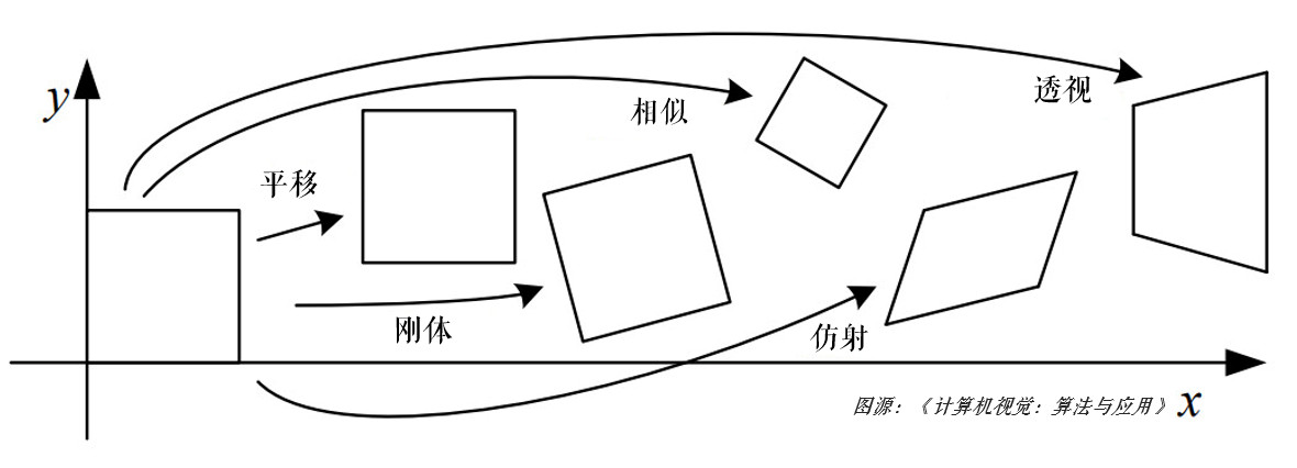
常见的 2D 图像变换从原理上讲主要包括基于 2×3 矩阵的仿射变换和基于 3×3 矩阵透视变换。
仿射变换
基本的图像变换就是二维坐标的变换:从一种二维坐标 (x,y) 到另一种二维坐标 (u,v) 的线性变换:
u=a1x+b1y+c1v=a2x+b2y+c2
如果写成矩阵的形式,就是:
[uv]=[a1a2b1b2][xy]+[c1c2]
作如下定义:
R=[a1a2b1b2],t=[c1c2],T=[Rt]
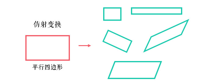
矩阵 T(2×3) 就称为仿射变换的变换矩阵,R 为线性变换矩阵,t 为平移矩阵,简单来说,仿射变换就是线性变换 + 平移。变换后直线依然是直线,平行线依然是平行线,直线间的相对位置关系不变,因此非共线的三个对应点便可确定唯一的一个仿射变换,线性变换 4 个自由度 + 平移 2 个自由度 →仿射变换自由度为 6。
来看下 OpenCV 中如何实现仿射变换:
import cv2
import numpy as np
import matplotlib.pyplot as plt
img = cv2.imread('drawing.jpg')
rows, cols = img.shape[:2]
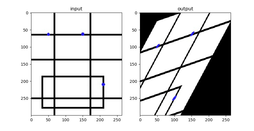
pts1 = np.float32([[50, 65], [150, 65], [210, 210]])
pts2 = np.float32([[50, 100], [150, 65], [100, 250]])
M = cv2.getAffineTransform(pts1, pts2)
dst = cv2.warpAffine(img, M, (cols, rows))
plt.subplot(121), plt.imshow(img), plt.title('input')
plt.subplot(122), plt.imshow(dst), plt.title('output')
plt.show()
三个点我已经在图中标记了出来。用cv2.getAffineTransform()生成变换矩阵,接下来再用cv2.warpAffine()实现变换。
思考:三个点我标记的是红色,为什么 Matplotlib 显示出来是下面这种颜色?(练习)
其实平移、旋转、缩放和翻转等变换就是对应了不同的仿射变换矩阵,下面分别来看下。
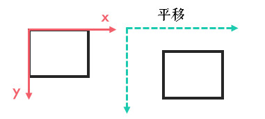
平移就是 x 和 y 方向上的直接移动,可以上下/左右移动,自由度为 2,变换矩阵可以表示为:
[uv]=[1001][xy]+[txty]
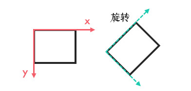
旋转是坐标轴方向饶原点旋转一定的角度 θ,自由度为 1,不包含平移,如顺时针旋转可以表示为:
[uv]=[cosθsinθ−sinθcosθ][xy]+[00]
思考:如果不是绕原点,而是可变点,自由度是多少呢?(请看下文刚体变换)
翻转是 x 或 y 某个方向或全部方向上取反,自由度为 2,比如这里以垂直翻转为例:
[uv]=[100−1][xy]+[00]
刚体变换
旋转 + 平移也称刚体变换(Rigid Transform),就是说如果图像变换前后两点间的距离仍然保持不变,那么这种变化就称为刚体变换。刚体变换包括了平移、旋转和翻转,自由度为 3。变换矩阵可以表示为:
[uv]=[cosθsinθ−sinθcosθ][xy]+[txty]
由于只是旋转和平移,刚体变换保持了直线间的长度不变,所以也称欧式变换(变化前后保持欧氏距离)。
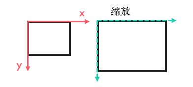
缩放是 x 和 y 方向的尺度(倍数)变换,在有些资料上非等比例的缩放也称为拉伸/挤压,等比例缩放自由度为 1,非等比例缩放自由度为 2,矩阵可以表示为:
[uv]=[sx00sy][xy]+[00]
相似变换
相似变换又称缩放旋转,相似变换包含了旋转、等比例缩放和平移等变换,自由度为 4。在 OpenCV 中,旋转就是用相似变换实现的:
若缩放比例为 scale,旋转角度为 θ,旋转中心是(centerx,centery),则仿射变换可以表示为:
[uv]=[α−ββα][xy]+[(1−α)centerx−βcenteryβcenterx+(1−α)centery]
其中,
α=scale⋅cosθ,β=scale⋅sinθ
相似变换相比刚体变换加了缩放,所以并不会保持欧氏距离不变,但直线间的夹角依然不变。
经验之谈:OpenCV 中默认按照逆时针旋转噢~
总结一下(原图[#计算机视觉:算法与应用 p39]):
| 变换 | 矩阵 | 自由度 | 保持性质 |
|---|
| 平移 | [I, t](2×3) | 2 | 方向/长度/夹角/平行性/直线性 |
| 刚体 | [R, t](2×3) | 3 | 长度/夹角/平行性/直线性 |
| 相似 | [sR, t](2×3) | 4 | 夹角/平行性/直线性 |
| 仿射 | [T](2×3) | 6 | 平行性/直线性 |
| 透视 | [T](3×3) | 8 | 直线性 |
透视变换
前面仿射变换后依然是平行四边形,并不能做到任意的变换。
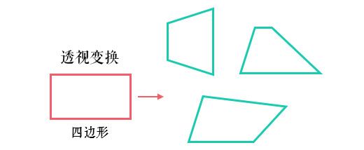
透视变换(Perspective Transformation)是将二维的图片投影到一个三维视平面上,然后再转换到二维坐标下,所以也称为投影映射(Projective Mapping)。简单来说就是二维 → 三维 → 二维的一个过程。
X=a1x+b1y+c1Y=a2x+b2y+c2Z=a3x+b3y+c3
这次我写成齐次矩阵的形式:
XYZ=a1a2a3b1b2b3c1c2c3xy1
其中,[a1a2b1b2]表示线性变换,[a3b3]产生透视变换,其余表示平移变换,因此仿射变换是透视变换的子集。接下来再通过除以 Z 轴转换成二维坐标:
x’=ZX=a3x+b3y+c3a1x+b1y+c1
y’=ZY=a3x+b3y+c3a2x+b2y+c2
透视变换相比仿射变换更加灵活,变换后会产生一个新的四边形,但不一定是平行四边形,所以需要非共线的四个点才能唯一确定,原图中的直线变换后依然是直线。因为四边形包括了所有的平行四边形,所以透视变换包括了所有的仿射变换。
OpenCV 中首先根据变换前后的四个点用cv2.getPerspectiveTransform()生成 3×3 的变换矩阵,然后再用cv2.warpPerspective()进行透视变换。实战演练一下:
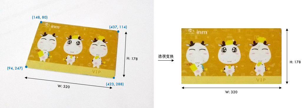
img = cv2.imread('card.jpg')
pts1 = np.float32([[148, 80], [437, 114], [94, 247], [423, 288]])
pts2 = np.float32([[0, 0], [320, 0], [0, 178], [320, 178]])
M = cv2.getPerspectiveTransform(pts1, pts2)
dst = cv2.warpPerspective(img, M, (320, 178))
plt.subplot(121), plt.imshow(img[:, :, ::-1]), plt.title('input')
plt.subplot(122), plt.imshow(dst[:, :, ::-1]), plt.title('output')
plt.show()
代码中有个img[:, :, ::-1]还记得吗?忘记的话,请看练习。
当然,我们后面学习了特征提取之后,就可以自动识别角点了。透视变换是一项很酷的功能。比如我们经常会用手机去拍身份证和文件,无论你怎么拍,貌似都拍不正或者有边框。如果你使用过手机上面一些扫描类软件,比如"扫描全能王","Office Lens",它们能很好地矫正图片,这些软件就是应用透视变换实现的。
- 请复习:无损保存和 Matplotlib 使用。